Clustering with Prostate Cancer

Final for Unsupervised Learning

Rohan Lewis

2021.03.24

Complete code can be found here. Click graphs and plots for full size.

I. Introduction

According to the American Cancer Society,

Other than skin cancer, prostate cancer is the most common cancer in American men. The American Cancer Society’s estimates for prostate cancer in the United States for 2021 are:

• About 248,530 new cases of prostate cancer.
• About 34,130 deaths from prostate cancer.

In addition:

• About 1 man in 8 will be diagnosed with prostate cancer during his lifetime.
• Prostate cancer is the second leading cause of cancer death in American men, behind only lung cancer.
• About 1 man in 41 will die of prostate cancer.

II. Main Objectives

The objective of this study is cluster groups of men based off metrics related to prostate and reproductive health.

Similarities within clusters and differences between clusters will be discussed.

III. Data

The data chosen was from a statistical set. The prostate data contains 97 observations and 9 metrics. They are as follows:

• lcavol - log cancer volume
• lweight - log prostate weight
• age - in years
• lbph - log of the amount of benign prostatic hyperplasia
• svi - seminal vesicle invasion
• lcp- log of capsular penetration
• gleason - a numeric vector
• pgg45 - percent of Gleason score 4 or 5
• lpsa - log prostate-specific antigen

The original study can be found here.

Here are some Key Statistics for Prostate Cancer from the American Cancer Society.

Clustering groups of men together that have similar characteristics, differentiating them from other clusters, may prove to be useful in various treatments in various stages of illnesses related to men's health.

IV. Exploratory Data Analysis

There were no missing values and several variables had already been log transformed.

1. Distributions and Histograms

Age is left skewed.

logCV, logPSA, and logPW have been appropriately log transformed and are close to normal distribution.

logBPH, logCP, and Gleason2 all have over 40% of their observations in the least value bin.

Gleason1 and SVI are both categorical and are unbalanced.

2. Correlations

Gleason1 and Gleason2 have the highest correlation at around 0.75.

logCV and logPSA, logCP and logCV, and logCP and SVI also have high correlations.

No variables will be removed, as multicollinearity is not an issue.

V. Clustering Models

The data will be split into training (70%) and validation (30%) sets.

I am using three usupervised learning algorithms:

• K-Means Clustering - comparing 1 to 10 clusters. An elbow plot will be used to determine the optimal cluster size.
• Hierarchical Agglomerative Clustering - using the euclidean for affinity and ward for linkage. The result is expressed as a dendrogram.
• MeanShift Clustering

For each of the three models, the cluster results of the train set will be represented as the color in a grid of pair-plots for all nine variables.

1. KMeans Clustering

The distortion and inertia imply n = 3 clusters is an appropriate value.

Pair-plots are shown below.

Cluster 2 has noticeable, tight peaks for logBPH, logPW, Gleason2, Gleason1, and SVI. Most of the variables have much overlap among the clusters.

2. Hierarchical Agglomerative Clustering

Below is a graphic of how the observations in the training set clustered together.

The colors of the above dendogram match with the clusters in the pair-plots shown below.

Again, most of the variables have much overlap among the clusters.

3. MeanShift Clustering

Pair-plots are shown below

MeanShift resulted in only two clusters. Again, most of the variables have much overlap among the clusters.

VI. Key Findings

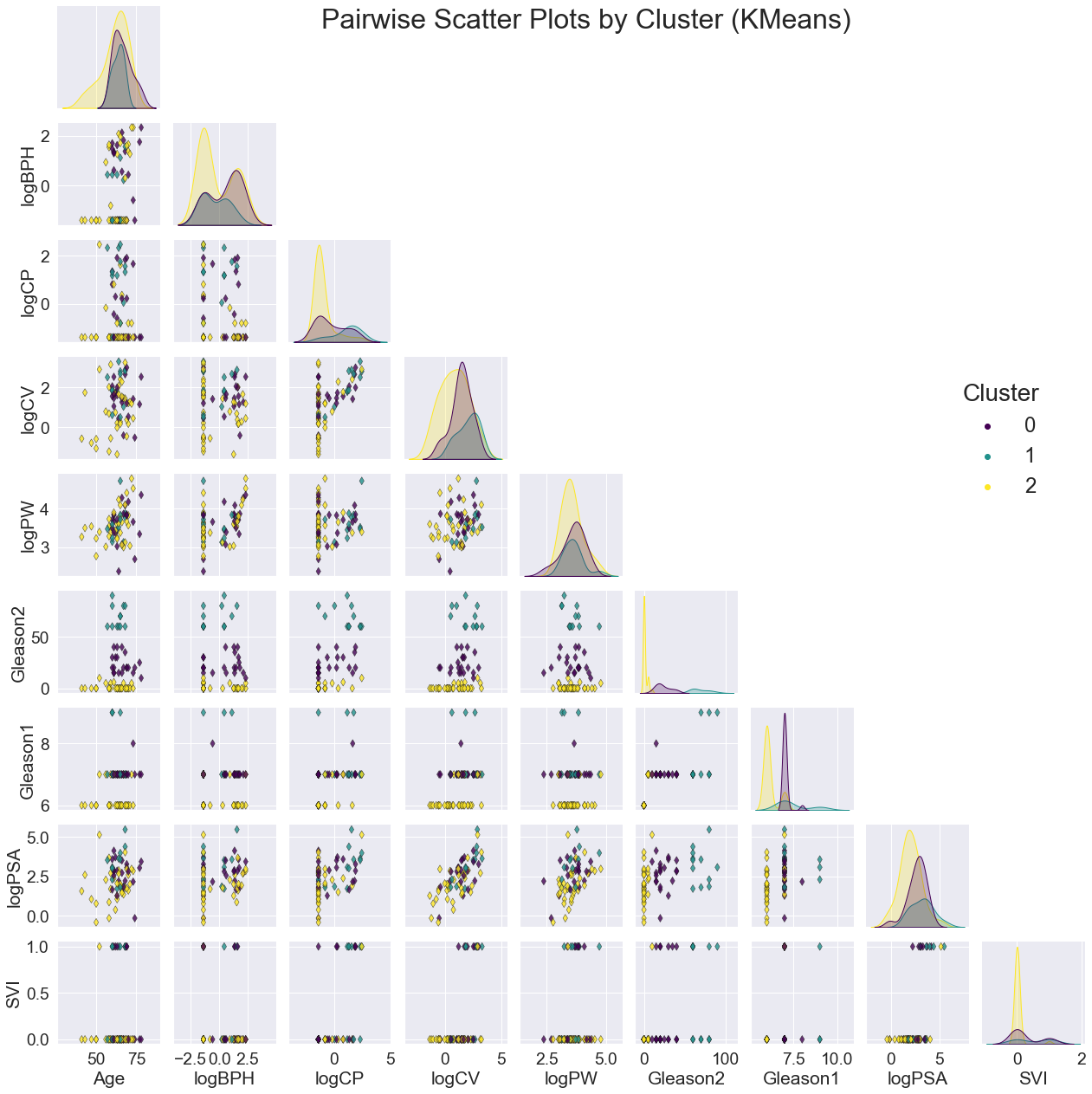
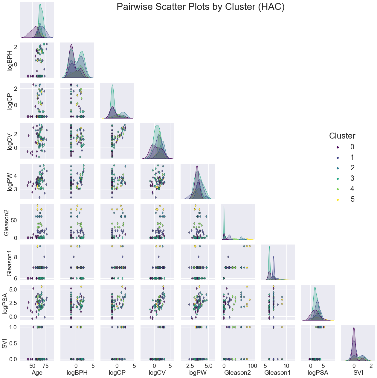
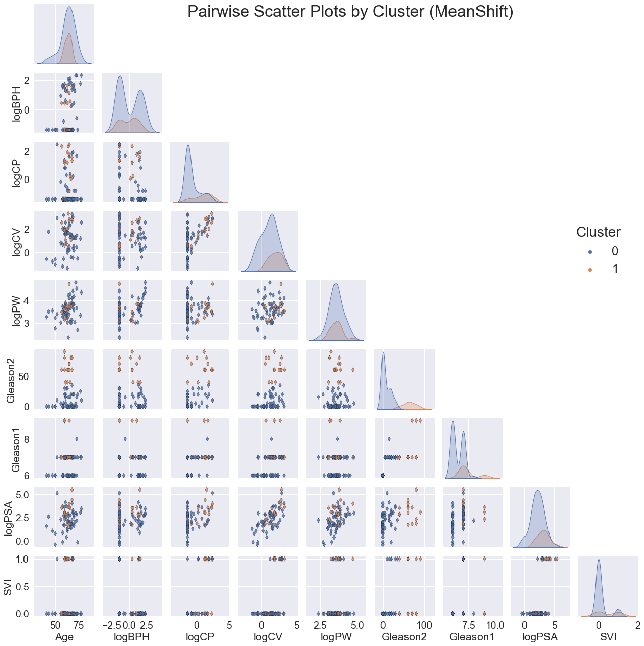
For all three models, the clusters seem to be most noticeably correlated with Gleason2. This is clear not only from the scatter plots of variable pairs, but the distinct separations in the distribution plot of Gleason2 along the diagonal.

Although there were a few peaks for the other variables, the overall distributions were generally highly overlapping. The scatter plots also had no emerging patterns.

VII. Final Model Selection

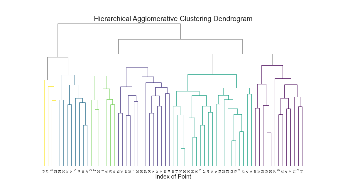
I choose Hierarchical Agglomerative Clustering as my final model. I chose it because I could set the cluster size from the dendogram and because it is recommended for uneven cluster sizes.

The validation pair-plots are shown below.

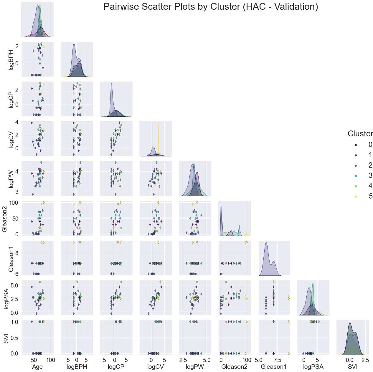
Again, the clusters are noticeably correlated with Gleason2. Perhaps Gleason2 is a good 'average' metric of the rest, which would explain more variance of the other variables among the clusters.

VIII. Conclusion, Next Steps, and Shortcomings

The dataset was only 97 observations and 9 variables. Only 67 observations were used in the clustering algorithms. More observations would have more diversity and perhaps more distinct clusters emerging.

Besides a few hours of reading some websites, I have very little subject knowledge of prostate health. I am certain there are many interactions, and perhaps other variables that I am unaware of which would be useful in clustering

Several variables were already log transformed. Would keeping their original values be more useful in clustering?

I did not fully test different affinities, linkages, or cluster numbers for the Hierarchical Agglomerative Clustering Algorithm. It is possible that some other combination of these parameters/hyperparameters would have more accurate clusters for diagnosis and treatment. A more in-depth look at the algorithm with subject knowledge would be very useful for better clustering.