Supervised Learning with Prostate Cancer
Final for Supervised Learning: Classification
Rohan Lewis
2021.07.13
Complete code can be found here. Click graphs and plots for full size.
I. Introduction
According to the American Cancer Society,
Other than skin cancer, prostate cancer is the most common cancer in American men. The American Cancer Society’s estimates for prostate cancer in the United States for 2021 are:
- About 248,530 new cases of prostate cancer.
- About 34,130 deaths from prostate cancer.
In addition:
- About 1 man in 8 will be diagnosed with prostate cancer during his lifetime.
- Prostate cancer is the second leading cause of cancer death in American men, behind only lung cancer.
- About 1 man in 41 will die of prostate cancer.
II. Main Objectives
The objective of this study is to predict various outcomes. Here are some questions that will be answered.
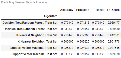
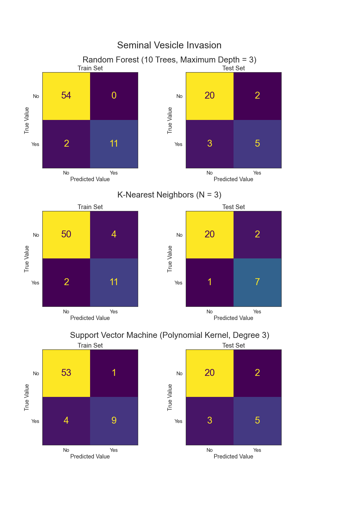
- Can Seminal Vesicle Invasion be predicted from other variables?
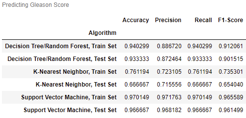
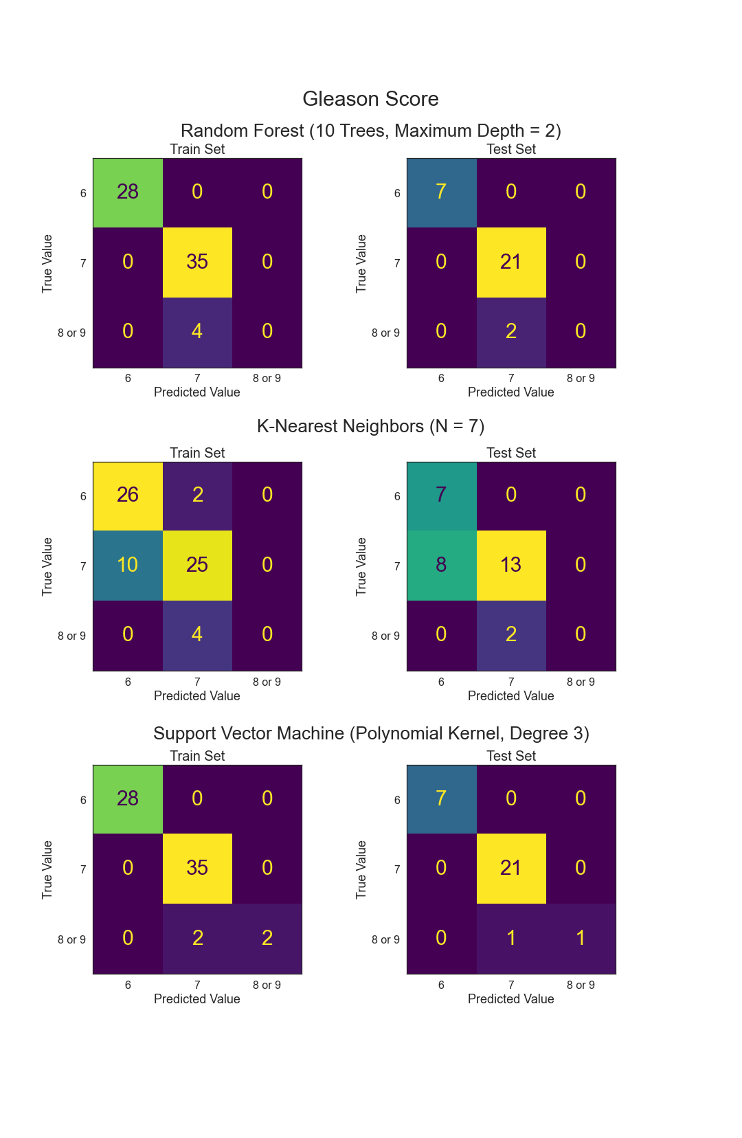
- Can Gleason Score be predicted from other variables?
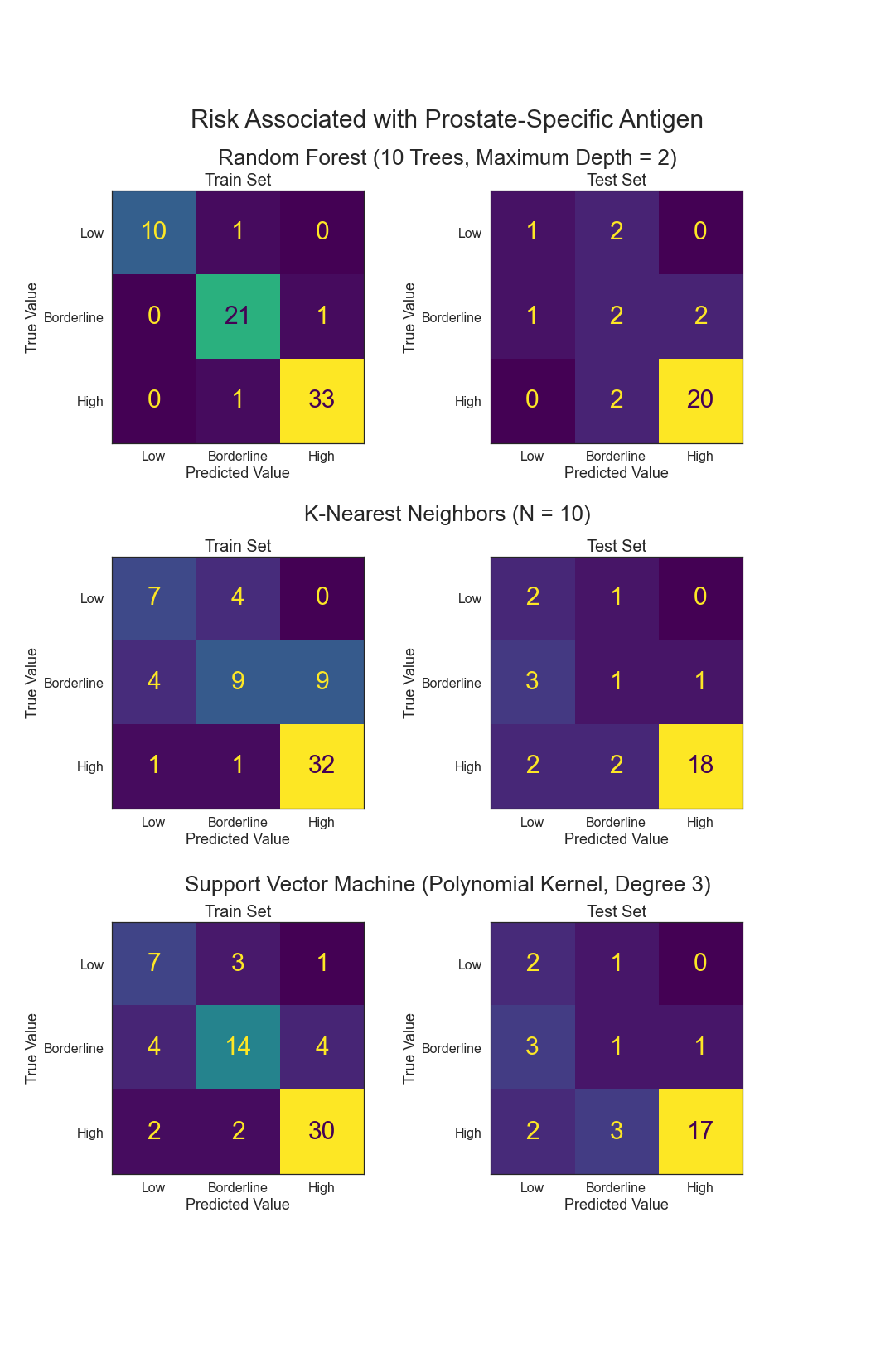
- Can Prostate-Specific Antigen levels be predicted from other variables?
III. Data
The data chosen was from a statistical set. The prostate data contains 97 observations and 9 metrics. They are as follows:
- lcavol - log cancer volume
- lweight - log prostate weight
- age - in years
- lbph - log of the amount of benign prostatic hyperplasia
- svi - seminal vesicle invasion
- lcp- log of capsular penetration
- gleason - a numeric vector
- pgg45 - percent of Gleason score 4 or 5
- lpsa - log prostate-specific antigen
The original study can be found here.
Here are some Key Statistics for Prostate Cancer from the American Cancer Society.
IV. Exploratory Data Analysis
There were no missing values and several variables had already been log transformed.
1. Distributions and Histograms
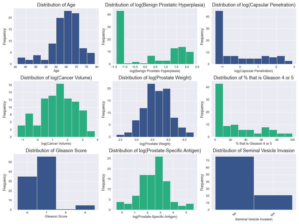
Age is left skewed.
logCV, logPSA, and logPW have been appropriately log transformed and are close to normal distribution.
logBPH, logCP, and Gleason2 all have over 40% of their observations in the least value bin.
Gleason1 and SVI are both categorical and are unbalanced.
2. Correlations
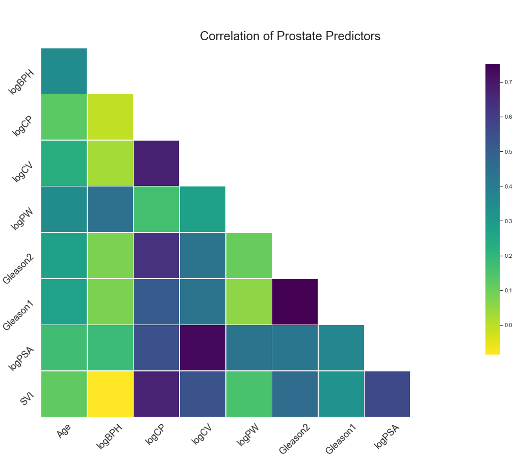
Gleason1 and Gleason2 have the highest correlation at around 0.75.
logCV and logPSA, logCP and logCV, and logCP and SVI also have high correlations.
No variables will be removed, as multicollinearity is not an issue.


.png)
.png)
.png)